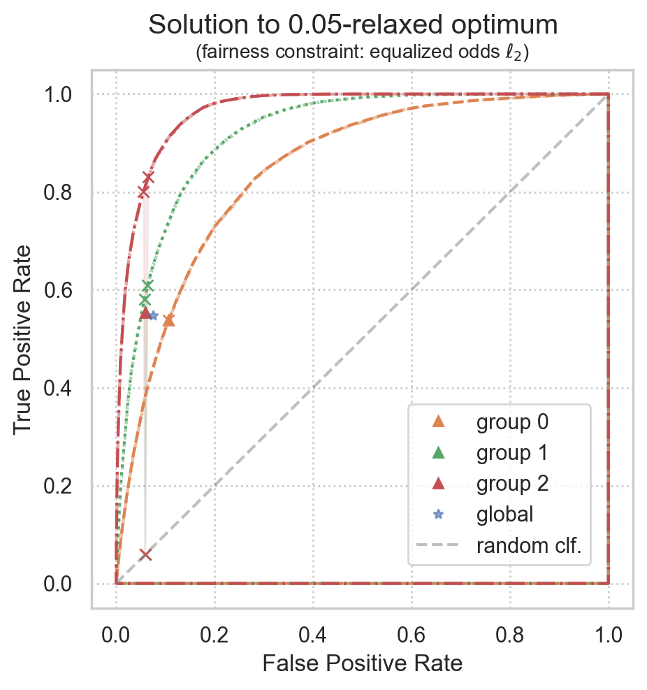
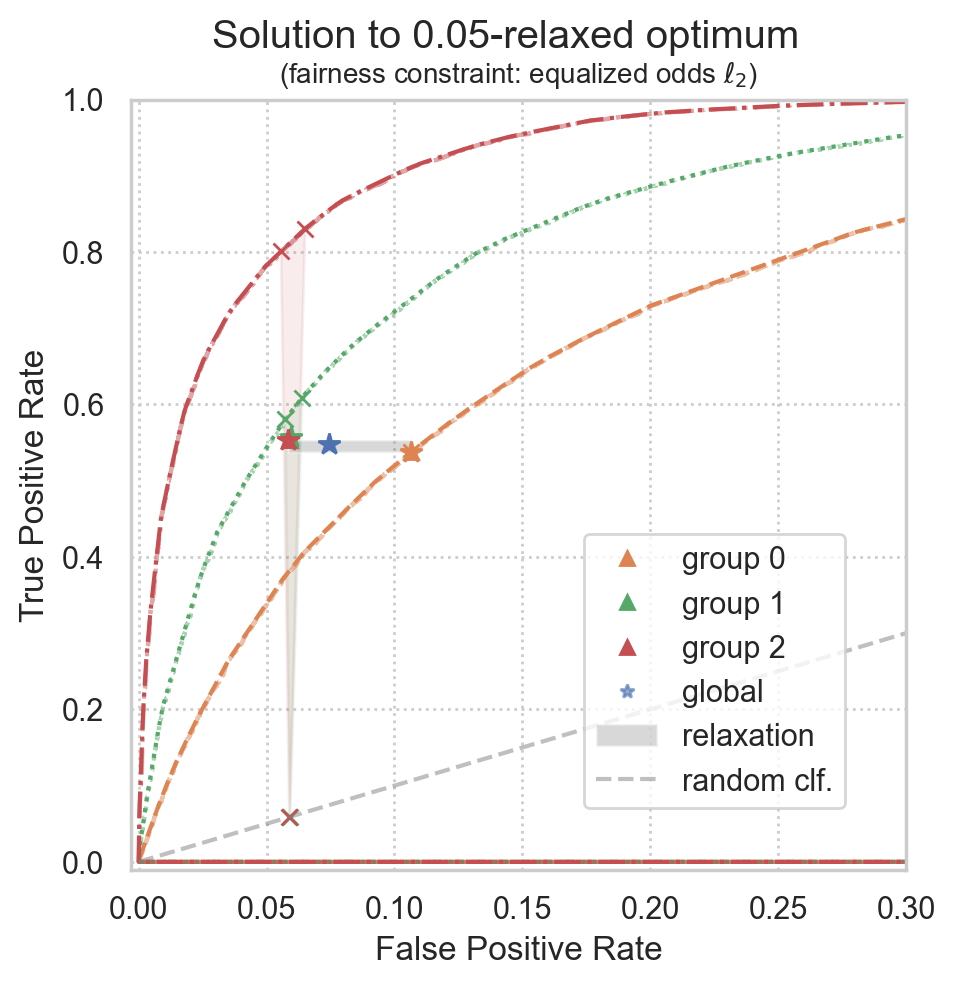
Achieving equalized odds on synthetic data

NOTE: this notebook has extra requirements, install them with:

pip install "error_parity[dev]"

import logging
from itertools import product

import numpy as np
import cvxpy as cp
from scipy.spatial import ConvexHull
from sklearn.metrics import roc_curve

from error_parity import __version__
print(f"Notebook ran using `error-parity=={__version__}`")

Notebook ran using `error-parity==0.3.11`

Given some data (X, Y, S)

def generate_synthetic_data(n_samples: int, n_groups: int, prevalence: float, seed: int):
    """Helper to generate synthetic features/labels/predictions."""

    # Construct numpy rng
    rng = np.random.default_rng(seed)

    # Different levels of gaussian noise per group (to induce some inequality in error rates)
    group_noise = [0.1 + 0.3 * rng.random() / (1+idx) for idx in range(n_groups)]

    # Generate predictions
    assert 0 < prevalence < 1
    y_score = rng.random(size=n_samples)

    # Generate labels
    # - define which samples belong to each group
    # - add different noise levels for each group
    group = rng.integers(low=0, high=n_groups, size=n_samples)

    y_true = np.zeros(n_samples)
    for i in range(n_groups):
        group_filter = group == i
        y_true_groupwise = ((
            y_score[group_filter] +
            rng.normal(size=np.sum(group_filter), scale=group_noise[i])
        ) > (1-prevalence)).astype(int)

        y_true[group_filter] = y_true_groupwise

    ### Generate features: just use the sample index
    # As we already have the y_scores, we can construct the features X
    # as the index of each sample, so we can construct a classifier that
    # simply maps this index to our pre-generated predictions for this clf.
    X = np.arange(len(y_true)).reshape((-1, 1))

    return X, y_true, y_score, group

# N_GROUPS = 4
N_GROUPS = 3

# N_SAMPLES = 1_000_000
N_SAMPLES = 100_000

SEED = 23

X, y_true, y_score, group = generate_synthetic_data(
    n_samples=N_SAMPLES,
    n_groups=N_GROUPS,
    prevalence=0.25,
    seed=SEED)

actual_prevalence = np.sum(y_true) / len(y_true)
print(f"Actual global prevalence: {actual_prevalence:.1%}")

Actual global prevalence: 26.6%

EPSILON_TOLERANCE = 0.05

FALSE_POS_COST = 1
FALSE_NEG_COST = 1

# L_P_NORM = np.inf
L_P_NORM = 2

---

Given a trained predictor (that outputs real-valued scores)

# Example predictor that predicts the synthetically produced scores above
predictor = lambda idx: y_score[idx]

Construct the fair optimal classifier (derived from the given predictor)

• Fairness is measured by the equal odds constraint (equal FPR and TPR among groups);

  • optionally, this constraint can be relaxed by some small tolerance;

• Optimality is measured as minimizing the expected loss,

  • parameterized by the given cost of false positive and false negative errors;

from error_parity import RelaxedThresholdOptimizer

postproc_clf = RelaxedThresholdOptimizer(
    predictor=predictor,
    constraint="equalized_odds",
    tolerance=EPSILON_TOLERANCE,
    false_pos_cost=FALSE_POS_COST,
    false_neg_cost=FALSE_NEG_COST,
    l_p_norm=L_P_NORM,
    max_roc_ticks=None,
    seed=SEED,
)

%%time
import logging
logging.basicConfig(level=logging.INFO, force=True)
postproc_clf.fit(X=X, y=y_true, group=group)

INFO:root:ROC convex hull contains 0.8% of the original points.
INFO:root:ROC convex hull contains 1.1% of the original points.
INFO:root:ROC convex hull contains 1.7% of the original points.
INFO:root:cvxpy solver took 0.000574791s; status is optimal.
INFO:root:Optimal solution value: 0.17475045311134396
INFO:root:Variable Global ROC point: value [0.07436224 0.54775546]
INFO:root:Variable ROC point for group 0: value [0.10639373 0.53750647]
INFO:root:Variable ROC point for group 1: value [0.05919955 0.55402037]
INFO:root:Variable ROC point for group 2: value [0.05891875 0.55319488]

CPU times: user 199 ms, sys: 8.76 ms, total: 208 ms
Wall time: 1.6 s

<error_parity.threshold_optimizer.RelaxedThresholdOptimizer at 0x11df428c0>

Plot solution

from matplotlib import pyplot as plt
import seaborn as sns
sns.set(style="whitegrid", rc={'grid.linestyle': ':'})

from error_parity.plotting import plot_postprocessing_solution

plot_postprocessing_solution(
    postprocessed_clf=postproc_clf,
    plot_roc_curves=True,
    plot_roc_hulls=True,
    dpi=200, figsize=(5, 5),
)
plt.show()

---

Plot realized ROC points

realized ROC points will converge to the theoretical solution for larger datasets, but some variance is expected for smaller datasets

# Set group-wise colors and global color
palette = sns.color_palette(n_colors=N_GROUPS + 1)
global_color = palette[0]
all_group_colors = palette[1:]

from error_parity.roc_utils import compute_roc_point_from_predictions

plot_postprocessing_solution(
    postprocessed_clf=postproc_clf,
    plot_roc_curves=True,
    plot_roc_hulls=True,
    plot_relaxation=True,
    dpi=200, figsize=(5, 5),
)

# Compute predictions
y_pred_binary = postproc_clf(X, group=group)

# Plot the group-wise points found
realized_roc_points = list()
for idx in range(N_GROUPS):

    # Evaluate triangulation of target point as a randomized clf
    group_filter = group == idx

    curr_realized_roc_point = compute_roc_point_from_predictions(y_true[group_filter], y_pred_binary[group_filter])
    realized_roc_points.append(curr_realized_roc_point)

    plt.plot(
        curr_realized_roc_point[0], curr_realized_roc_point[1],
        color=all_group_colors[idx],
        marker="*", markersize=8,
        lw=0,
    )

realized_roc_points = np.vstack(realized_roc_points)

# Plot actual global classifier performance
global_clf_realized_roc_point = compute_roc_point_from_predictions(y_true, y_pred_binary)
plt.plot(
    global_clf_realized_roc_point[0], global_clf_realized_roc_point[1],
    color=global_color,
    marker="*", markersize=8,
    lw=0,
)

plt.xlim(-0.003, 0.3)
plt.ylim(-0.01, 1.0)

plt.show()

Compute distances between theorized ROC points and empirical ROC points

# Distances to group-wise targets:
for i, (target_point, actual_point) in enumerate(zip(postproc_clf.groupwise_roc_points, realized_roc_points)):
    dist = np.linalg.norm(target_point - actual_point, ord=2)
    print(f"Group {i}: l2 distance from target to realized point := {dist:.3%}")

# Distance to global target point:
dist = np.linalg.norm(postproc_clf.global_roc_point - global_clf_realized_roc_point, ord=2)
print(f"Global l2 distance from target to realized point   := {dist:.3%}")

Group 0: l2 distance from target to realized point := 0.000%
Group 1: l2 distance from target to realized point := 0.282%
Group 2: l2 distance from target to realized point := 0.063%
Global l2 distance from target to realized point   := 0.089%

Compute performance differences

assumes FP_cost == FN_cost == 1.0

from sklearn.metrics import accuracy_score
from error_parity.roc_utils import calc_cost_of_point

# Empirical
accuracy_val = accuracy_score(y_true, y_pred_binary)

# Theoretical
theoretical_global_cost = calc_cost_of_point(
    fpr=postproc_clf.global_roc_point[0],
    fnr=1 - postproc_clf.global_roc_point[1],
    prevalence=y_true.sum() / len(y_true),
)

print(f"Actual accuracy: \t\t\t{accuracy_val:.3%}")
print(f"Actual error rate (1 - Acc.):\t\t{1 - accuracy_val:.3%}")
print(f"Theoretical cost of solution found:\t{theoretical_global_cost:.3%}")

Actual accuracy:                        82.559%
Actual error rate (1 - Acc.):           17.441%
Theoretical cost of solution found:     17.475%

print(f"Accuracy for dummy constant classifier: {max(np.mean(y_true==label) for label in {0, 1}):.1%}")

Accuracy for dummy constant classifier: 73.4%

from error_parity.evaluation import eval_accuracy_and_equalized_odds
lp_acc, lp_eq_odds = eval_accuracy_and_equalized_odds(y_true, y_pred_binary, group, l_p_norm=L_P_NORM)

print(f"Realized LP accuracy:\t {lp_acc:.1%}")
print(f"Realized LP eq. odds violation: {lp_eq_odds:.1%}\n")

Realized LP accuracy:    82.6%
Realized LP eq. odds violation: 5.1%

Plot postprocessing Pareto frontier

i.e., all attainable optimal trade-offs for this predictor

from error_parity.pareto_curve import compute_postprocessing_curve

postproc_results_df = compute_postprocessing_curve(
    model=predictor,
    fit_data=(X, y_true, group),
    eval_data={
        "fit": (X, y_true, group),
    },
    fairness_constraint="equalized_odds",
    l_p_norm=L_P_NORM,
    bootstrap=True,
    seed=SEED,
    predict_method="__call__",
)

INFO:root:Using `n_jobs=9` to compute adjustment curve.
INFO:root:Computing postprocessing for the following constraint tolerances: [0.   0.01 0.02 0.03 0.04 0.05 0.06 0.07 0.08 0.09 0.1  0.11 0.12 0.13
 0.14 0.15 0.16 0.17 0.18 0.19 0.2  0.3  0.4  0.5  0.6  0.7  0.8  0.9 ].

from error_parity.plotting import plot_postprocessing_frontier
from matplotlib import pyplot as plt

plot_postprocessing_frontier(
    postproc_results_df,
    perf_metric="accuracy",
    disp_metric=f"equalized_odds_diff_l{postproc_clf.l_p_norm}",
    show_data_type="fit",
    constant_clf_perf=max((y_true == const_pred).mean() for const_pred in {0, 1}),
    model_name=r"$\bigstar$",
)

plt.xlabel(r"accuracy $\rightarrow$")
l_p_norm_str = str(postproc_clf.l_p_norm) if postproc_clf.l_p_norm != np.inf else r"\infty"
plt.ylabel(r"equalized odds $\ell_" + l_p_norm_str + r"$ violation $\leftarrow$")
plt.show()