Achieving equalized odds on real-world ACS data (ACSIncome)

NOTE: this notebook has extra requirements, install them with: pip install "error_parity[dev]"

DATA: the data used in this notebook can be easily downloaded and parsed using the companion notebook parse-folktables-datasets.ipynb;

import logging
from itertools import product
from pathlib import Path

import pandas as pd
import numpy as np
import cvxpy as cp
from scipy.spatial import ConvexHull
from sklearn.metrics import roc_curve

from error_parity import __version__
print(f"Notebook ran using `error-parity=={__version__}`")

Notebook ran using `error-parity==0.3.11`

Given some data (X, Y, S)

ACS_TASK = "ACSIncome"
SEED = 42

data_dir = Path("~").expanduser() / "data" / "folktables" / "train=0.6_test=0.2_validation=0.2_max-groups=4"

ACS_CATEGORICAL_COLS = {
    'COW',  # class of worker
    'MAR',  # marital status
    'OCCP', # occupation code
    'POBP', # place of birth code
    'RELP', # relationship status
    'SEX',
    'RAC1P', # race code
    'DIS',  # disability
    'ESP',  # employment status of parents
    'CIT',  # citizenship status
    'MIG',  # mobility status
    'MIL',  # military service
    'ANC',  # ancestry
    'NATIVITY',
    'DEAR',
    'DEYE',
    'DREM',
    'ESR',
    'ST',
    'FER',
    'GCL',
    'JWTR',
#     'PUMA',
#     'POWPUMA',
}

import folktables

def split_X_Y_S(data, label_col: str, sensitive_col: str, ignore_cols=None, unawareness=False) -> tuple:
    ignore_cols = ignore_cols or []
    ignore_cols.append(label_col)
    if unawareness:
        ignore_cols.append(sensitive_col)

    feature_cols = [c for c in data.columns if c not in ignore_cols]

    return (
        data[feature_cols],                           # X
        data[label_col].to_numpy().astype(int),       # Y
        data[sensitive_col].to_numpy().astype(int),   # S
    )

def load_ACS_data(dir_path: str, task_name: str, sensitive_col: str = None) -> pd.DataFrame:
    """Loads the given ACS task data from pre-generated datasets.

    Returns
    -------
    dict[str, tuple]
        A list of tuples, each tuple composed of (features, label, sensitive_attribute).
        The list is sorted as follows" [<train data tuple>, <test data tuple>, <val. data tuple>].
    """
    # Load task object
    task_obj = getattr(folktables, task_name)

    # Load train, test, and validation data
    data = dict()
    for data_type in ['train', 'test', 'validation']:
        # Construct file path
        path = Path(dir_path) / f"{task_name}.{data_type}.csv"

        if not path.exists():
            print(f"Couldn't find data for '{path.name}' (this is probably expected).")
            continue

        # Read data from disk
        df = pd.read_csv(path, index_col=0)

        # Set categorical columns
        cat_cols = ACS_CATEGORICAL_COLS & set(df.columns)
        df = df.astype({col: "category" for col in cat_cols})

        data[data_type] = split_X_Y_S(
            df,
            label_col=task_obj.target,
            sensitive_col=sensitive_col or task_obj.group,
        )

    return data

# Load and pre-process data
all_data = load_ACS_data(
    dir_path=data_dir, task_name=ACS_TASK,
)

# Unpack into features, label, and group
X_train, y_train, s_train = all_data["train"]
X_test, y_test, s_test = all_data["test"]
if "validation" in all_data:
    X_val, y_val, s_val = all_data["validation"]
else:
    print("No validation data.")

n_groups = len(np.unique(s_train))

actual_prevalence = np.sum(y_train) / len(y_train)
print(f"Global prevalence: {actual_prevalence:.1%}")

Global prevalence: 37.2%

EPSILON_TOLERANCE = 0.05

FALSE_POS_COST = 1
FALSE_NEG_COST = 1

L_P_NORM = np.inf         # constrain l-infinity distance between ROC points
# L_P_NORM = 1            # constrain l-1 distance between ROC points
# L_P_NORM = 2            # constrain l-2 distance between ROC points

---

Given a trained predictor (that outputs real-valued scores)

from sklearn.ensemble import RandomForestClassifier

rf_clf = RandomForestClassifier(n_jobs=-2)

%%time
rf_clf.fit(X_train, y_train)

CPU times: user 1min 46s, sys: 1.81 s, total: 1min 47s
Wall time: 13.7 s

RandomForestClassifier(n_jobs=-2)

In a Jupyter environment, please rerun this cell to show the HTML representation or trust the notebook.
On GitHub, the HTML representation is unable to render, please try loading this page with nbviewer.org.

predictor = lambda X: rf_clf.predict_proba(X)[:, -1]

Construct the fair optimal classifier (derived from the given predictor)

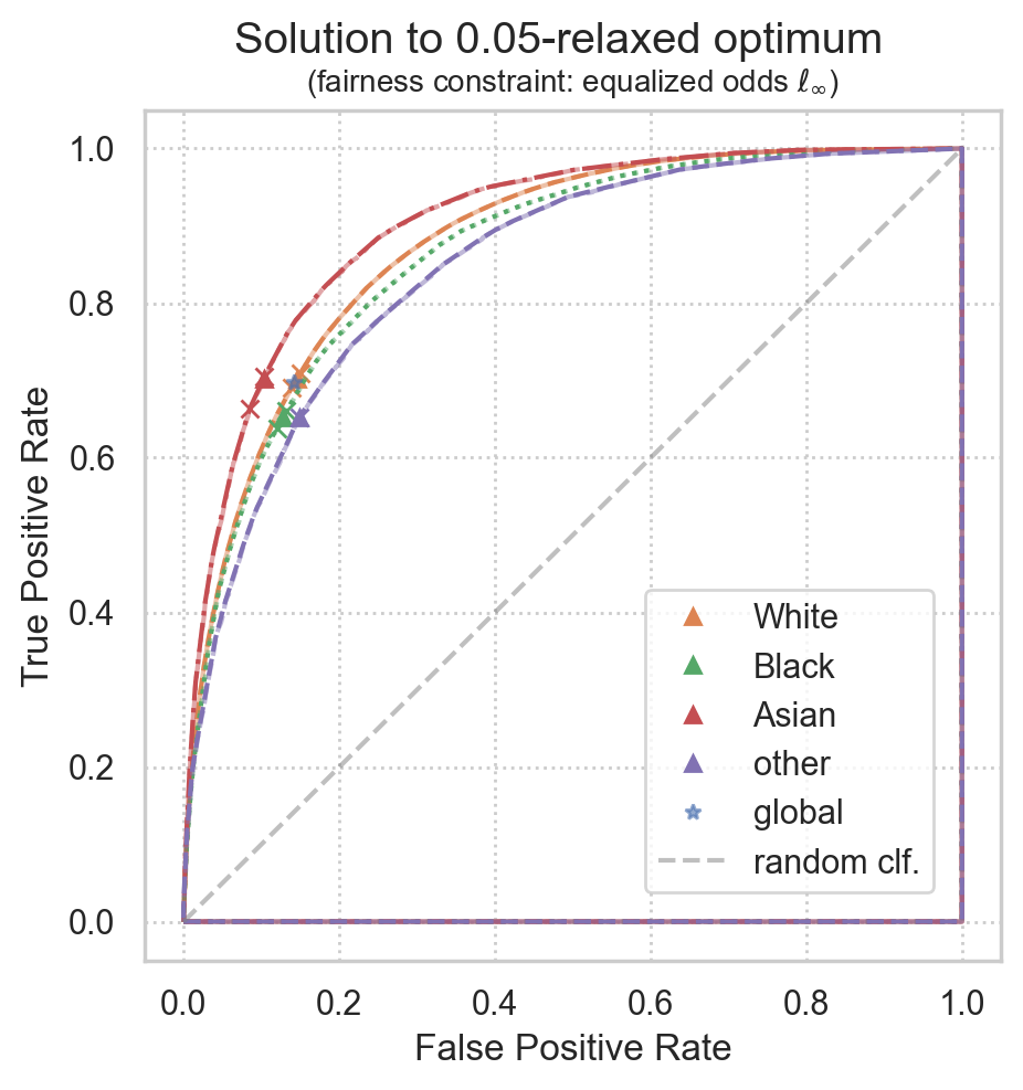
• Fairness is measured by the equal odds constraint (equal FPR and TPR among groups);

  • optionally, this constraint can be relaxed by some small tolerance;

  • the type of relaxation can be changed using the l_p_norm key-word argument (default is l_p_norm=np.inf);

• Optimality is measured as minimizing the expected loss while fulfilling the fairness constraint,

  • parameterized by the given cost of false positive and false negative errors;

if "validation" in all_data:
    X_fit, y_fit, s_fit = X_val, y_val, s_val
else:
    X_fit, y_fit, s_fit = X_train, y_train, s_train

from error_parity import RelaxedThresholdOptimizer

postproc_clf = RelaxedThresholdOptimizer(
    predictor=predictor,
    constraint="equalized_odds",
    tolerance=EPSILON_TOLERANCE,
    false_pos_cost=FALSE_POS_COST,
    false_neg_cost=FALSE_NEG_COST,
    l_p_norm=L_P_NORM,
    seed=SEED,
)

%%time
import logging
logging.basicConfig(level=logging.INFO, force=True)
postproc_clf.fit(X=X_fit, y=y_fit, group=s_fit)

INFO:root:ROC convex hull contains 8.7% of the original points.
INFO:root:ROC convex hull contains 10.8% of the original points.
INFO:root:ROC convex hull contains 6.0% of the original points.
INFO:root:ROC convex hull contains 9.6% of the original points.
INFO:root:cvxpy solver took 0.00044025s; status is optimal.
INFO:root:Optimal solution value: 0.201182803373743
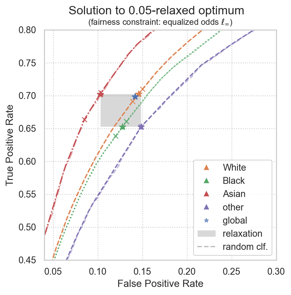
INFO:root:Variable Global ROC point: value [0.14162381 0.69846535]
INFO:root:Variable ROC point for group 0: value [0.14576582 0.70242546]
INFO:root:Variable ROC point for group 1: value [0.12760711 0.65242546]
INFO:root:Variable ROC point for group 2: value [0.10263456 0.70242546]
INFO:root:Variable ROC point for group 3: value [0.14840647 0.65242546]

CPU times: user 14.9 s, sys: 218 ms, total: 15.1 s
Wall time: 2.14 s

<error_parity.threshold_optimizer.RelaxedThresholdOptimizer at 0x163262380>

Plot solution

from matplotlib import pyplot as plt
import seaborn as sns
sns.set(style="whitegrid", rc={'grid.linestyle': ':'})

all_groups_name_map = {
    0: "White",
    1: "Black",
    2: "American Indian",
    3: "Alaska Native",
    4: "American Indian",
    5: "Asian",
    6: "Native Hawaiian",
    7: "other single race",
    8: "other multiple races",
}

largest_groups_name_map = {
    0: "White",
    1: "Black",
    2: "Asian",
    3: "other",
}

group_name_map=all_groups_name_map if len(np.unique(s_fit)) > len(largest_groups_name_map) else largest_groups_name_map

from error_parity.plotting import plot_postprocessing_solution
plot_postprocessing_solution(
    postprocessed_clf=postproc_clf,
    plot_roc_curves=True,
    plot_roc_hulls=True,
    dpi=200, figsize=(5, 5),
    group_name_map=group_name_map,
)
plt.show()

Theoretical results:

acc_val = 1 - postproc_clf.cost(1.0, 1.0)
unf_val = postproc_clf.constraint_violation()

print(f"Accuracy:   {acc_val:.1%}")
print(f"Unfairness: {unf_val:.1%} <= {EPSILON_TOLERANCE:.1%}")

INFO:root:Maximum fairness violation is between group=0 (p=[0.14576582 0.70242546]) and group=3 (p=[0.14840647 0.65242546]);

Accuracy:   79.9%
Unfairness: 5.0% <= 5.0%

---

Plot realized ROC points

Realized ROC points will converge to the theoretical solution for larger datasets, but some variance is expected for smaller datasets.

# Set group-wise colors and global color
palette = sns.color_palette(n_colors=n_groups + 1)
global_color = palette[0]
all_group_colors = palette[1:]

from error_parity.roc_utils import compute_roc_point_from_predictions

plot_postprocessing_solution(
    postprocessed_clf=postproc_clf,
    plot_roc_curves=True,
    plot_roc_hulls=True,
    plot_relaxation=True,
    dpi=200, figsize=(5, 5),
    group_name_map=group_name_map,
)

# Compute predictions
y_fit_preds = postproc_clf(X_fit, group=s_fit)

# Plot the group-wise points found
realized_roc_points = list()
for idx in range(n_groups):

    # Evaluate triangulation of target point as a randomized clf
    group_filter = s_fit == idx

    curr_realized_roc_point = compute_roc_point_from_predictions(y_fit[group_filter], y_fit_preds[group_filter])
    realized_roc_points.append(curr_realized_roc_point)

    plt.plot(
        curr_realized_roc_point[0], curr_realized_roc_point[1],
        color=all_group_colors[idx],
        marker="*", markersize=8,
        lw=0,
    )

realized_roc_points = np.vstack(realized_roc_points)

# Plot actual global classifier performance
global_clf_realized_roc_point = compute_roc_point_from_predictions(y_fit, y_fit_preds)
plt.plot(
    global_clf_realized_roc_point[0], global_clf_realized_roc_point[1],
    color=global_color,
    marker="*", markersize=8,
    lw=0,
)

plt.xlim(0.04, 0.3)
plt.ylim(0.45, 0.80)
plt.legend()

plt.show()

# Distances to group-wise targets:
for i, (target_point, actual_point) in enumerate(zip(postproc_clf.groupwise_roc_points, realized_roc_points)):
    dist = np.linalg.norm(target_point - actual_point, ord=2)
    print(f"Group {i}: l2 distance from target to realized point := {dist:.3%} (size={np.sum(s_fit==i)})")

# Distance to global target point:
dist = np.linalg.norm(postproc_clf.global_roc_point - global_clf_realized_roc_point, ord=2)
print(f"Global l2 distance from target to realized point   := {dist:.3%}")

Group 0: l2 distance from target to realized point := 0.010% (size=259521)
Group 1: l2 distance from target to realized point := 0.017% (size=29518)
Group 2: l2 distance from target to realized point := 0.052% (size=19386)
Group 3: l2 distance from target to realized point := 0.000% (size=12570)
Global l2 distance from target to realized point   := 0.007%

assumes FP_cost == FN_cost == 1.0

from sklearn.metrics import accuracy_score
from error_parity.roc_utils import calc_cost_of_point

# Empirical accuracy
accuracy_fit = accuracy_score(y_fit, y_fit_preds)

print(f"Actual accuracy: \t\t{accuracy_fit:.3%}")
print(f"Actual error rate (1 - Acc.):\t{1 - accuracy_fit:.3%}")
print(f"Theoretical error rate:\t\t{postproc_clf.cost(1.0, 1.0):.3%}")

Actual accuracy:                79.886%
Actual error rate (1 - Acc.):   20.114%
Theoretical error rate:         20.118%

---

from tqdm.auto import tqdm

# Compute prediction scores
y_test_scores = predictor(X_test)

acc_unfair_best, acc_unfair_threshold = max((accuracy_score(y_test, y_test_scores >= t), t) for t in tqdm(np.arange(0, 1, 2e-2)))
print(f"Best (train) unfair accuracy is {acc_unfair_best:.3%}, with threshold t={acc_unfair_threshold}")

Best (train) unfair accuracy is 80.208%, with threshold t=0.48

from error_parity.evaluation import eval_accuracy_and_equalized_odds
print("Best (unconstrained) single-threshold classifier:")

eval_accuracy_and_equalized_odds(
    y_true=y_test,
    y_pred_binary=predictor(X_test) >= acc_unfair_threshold,
    sensitive_attr=s_test,
    l_p_norm=L_P_NORM,
    display=True,
)

print("Best (constrained) multi-threshold classifier:")
eval_accuracy_and_equalized_odds(
    y_true=y_test,
    y_pred_binary=postproc_clf(X_test, group=s_test),
    sensitive_attr=s_test,
    l_p_norm=L_P_NORM,
    display=True,
);

Best (unconstrained) single-threshold classifier:
        Accuracy:   80.21%
        Unfairness: 35.50%
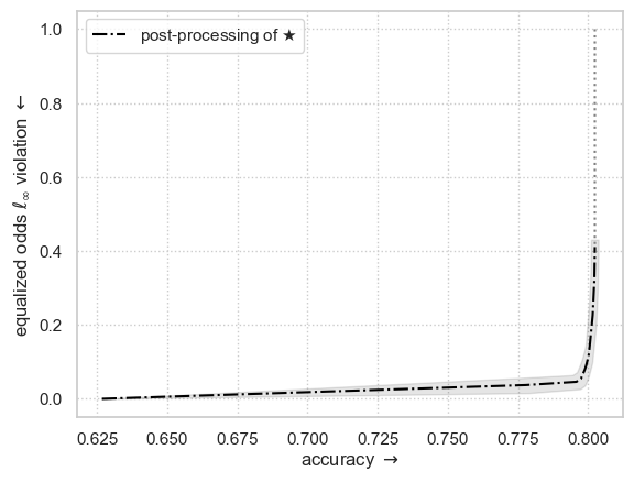
Best (constrained) multi-threshold classifier:
        Accuracy:   79.90%
        Unfairness: 8.10%

Fairness vs Performance trade-off

Plotting the entire Pareto frontier may take a few minutes…

from error_parity.pareto_curve import compute_postprocessing_curve

postproc_results_df = compute_postprocessing_curve(
    model=rf_clf,
    fit_data=(X_fit, y_fit, s_fit),
    eval_data={
        "test": (X_test, y_test, s_test),
    },
    fairness_constraint="equalized_odds",
    l_p_norm=L_P_NORM,
    tolerance_ticks=np.hstack((
        np.arange(0.0, 0.1, 1e-2),
        np.arange(0.1, 1.0, 1e-1),
    )),
    bootstrap=True,
    seed=SEED,
)

INFO:root:Using `n_jobs=9` to compute adjustment curve.
INFO:root:Computing postprocessing for the following constraint tolerances: [0.   0.01 0.02 0.03 0.04 0.05 0.06 0.07 0.08 0.09 0.1  0.2  0.3  0.4
 0.5  0.6  0.7  0.8  0.9 ].

from error_parity.plotting import plot_postprocessing_frontier
from matplotlib import pyplot as plt

plot_postprocessing_frontier(
    postproc_results_df,
    perf_metric="accuracy",
    disp_metric=f"equalized_odds_diff_l{postproc_clf.l_p_norm}",
    show_data_type="test",
    constant_clf_perf=max((y_test == const_pred).mean() for const_pred in {0, 1}),
    model_name=r"$\bigstar$",
)

plt.xlabel(r"accuracy $\rightarrow$")
l_p_norm_str = str(postproc_clf.l_p_norm) if postproc_clf.l_p_norm != np.inf else r"\infty"
plt.ylabel(r"equalized odds $\ell_" + l_p_norm_str + r"$ violation $\leftarrow$")
plt.show()

---

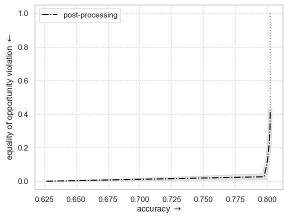
Fit and plot similar example but using “Equal Opportunity” fairness metric

equal opportunity is achieved by setting fairness_constraint="true_positive_rate_parity"

from error_parity.pareto_curve import compute_postprocessing_curve

postproc_results_df = compute_postprocessing_curve(
    model=rf_clf,
    fit_data=(X_fit, y_fit, s_fit),
    eval_data={
        "test": (X_test, y_test, s_test),
    },
    fairness_constraint="true_positive_rate_parity",
    tolerance_ticks=np.hstack((
        np.arange(0.0, 0.1, 1e-2),
        np.arange(0.1, 1.0, 1e-1),
    )),
    bootstrap=True,
    seed=SEED,
)

plot_postprocessing_frontier(
    postproc_results_df,
    perf_metric="accuracy",
    disp_metric="tpr_diff",
    show_data_type="test",
    constant_clf_perf=max((y_test == const_pred).mean() for const_pred in {0, 1}),
)

plt.xlabel(r"accuracy $\rightarrow$")
plt.ylabel(r"equality of opportunity violation $\leftarrow$")
plt.show()