Example usage of error-parity with other fairness-constrained classifiers
Contents:
Train a standard (unconstrained) model;
Check attainable fairness-accuracy trade-offs via post-processing, with the
error-paritypackage;Train fairness-constrained model (in-processing fairness intervention), with the
fairlearnpackage;Map results for post-processing + in-processing interventions;
NOTE: This notebook has the following extra requirements: fairlearn lightgbm.
Install them with pip install fairlearn lightgbm
[1]:
import os
import numpy as np
[2]:
from error_parity import __version__
print(f"error-parity=={__version__}")
error-parity==0.3.11
[3]:
from matplotlib import pyplot as plt
import seaborn as sns
sns.set(palette="colorblind", style="whitegrid", rc={"grid.linestyle": "--", "figure.dpi": 200, "figure.figsize": (4,3)})
Some useful global constants:
[4]:
SEED = 2

TEST_SIZE = 0.3
VALIDATION_SIZE = None

PERF_METRIC = "accuracy"
DISP_METRIC = "equalized_odds_diff"

N_JOBS = max(2, os.cpu_count() - 2)

np.random.seed(SEED)
Fetch UCI Adult data
We’ll use the sex column as the sensitive attribute. That is, false positive (FP) and false negative (FN) errors should not disproportionately impact individuals based on their sex.
[5]:
SENSITIVE_COL = "sex"
sensitive_col_map = {"Male": 0, "Female": 1}

# NOTE: You can also try to run this using the `race` column as sensitive attribute (as commented below).
# SENSITIVE_COL = "race"
# sensitive_col_map = {"White": 0, "Black": 1, "Asian-Pac-Islander": 1, "Amer-Indian-Eskimo": 1, "Other": 1}

sensitive_col_inverse = {val: key for key, val in sensitive_col_map.items()}

POS_LABEL = ">50K"
Download data.
[6]:
from fairlearn.datasets import fetch_adult

X, Y = fetch_adult(
    as_frame=True,
    return_X_y=True,
)

# Map labels and sensitive column to numeric data
Y = np.array(Y == POS_LABEL, dtype=int)
S = np.array([sensitive_col_map[elem] for elem in X[SENSITIVE_COL]], dtype=int)
Split in train/test/validation data.
[7]:
from sklearn.model_selection import train_test_split

X_train, X_other, y_train, y_other, s_train, s_other = train_test_split(
    X, Y, S,
    test_size=TEST_SIZE + (VALIDATION_SIZE or 0),
    stratify=Y, random_state=SEED,
)

if VALIDATION_SIZE is not None and VALIDATION_SIZE > 0:
    X_val, X_test, y_val, y_test, s_val, s_test = train_test_split(
        X_other, y_other, s_other,
        test_size=TEST_SIZE / (TEST_SIZE + VALIDATION_SIZE),
        stratify=y_other, random_state=SEED,
    )
else:
    X_test, y_test, s_test = X_other, y_other, s_other
    X_val, y_val, s_val = X_train, y_train, s_train
Log the accuracy attainable by a dummy constant classifier.
[8]:
def compute_constant_clf_accuracy(labels: np.ndarray) -> float:
    return max((labels == const_pred).mean() for const_pred in np.unique(labels))

constant_clf_accuracy = {
    "train": compute_constant_clf_accuracy(y_train),
    "test": compute_constant_clf_accuracy(y_test),
    "validation": compute_constant_clf_accuracy(y_val),
}
constant_clf_accuracy
[8]:
{'train': 0.7607125098715961,
 'test': 0.7607315908005187,
 'validation': 0.7607125098715961}
Train a standard (unconstrained) classifier
[9]:
from lightgbm import LGBMClassifier

unconstr_clf = LGBMClassifier(verbosity=-1)
unconstr_clf.fit(X_train, y_train)
[9]:
LGBMClassifier(verbosity=-1)In a Jupyter environment, please rerun this cell to show the HTML representation or trust the notebook.
On GitHub, the HTML representation is unable to render, please try loading this page with nbviewer.org.
LGBMClassifier(verbosity=-1)
[10]:
from error_parity.evaluation import evaluate_predictions_bootstrap

unconstr_test_results = evaluate_predictions_bootstrap(
    y_true=y_test,
    y_pred_scores=unconstr_clf.predict(X_test, random_state=SEED).astype(float),
    sensitive_attribute=s_test,
)

print(
    f"In-processing model: \n"
    f">       accuracy = {unconstr_test_results['accuracy_mean']:.3}\n"
    f"> equalized odds = {unconstr_test_results['equalized_odds_diff_mean']:.3}\n"
)
In-processing model:
>       accuracy = 0.87
> equalized odds = 0.0673
Map attainable fairness-accuracy trade-offs via (relaxed) post-processing
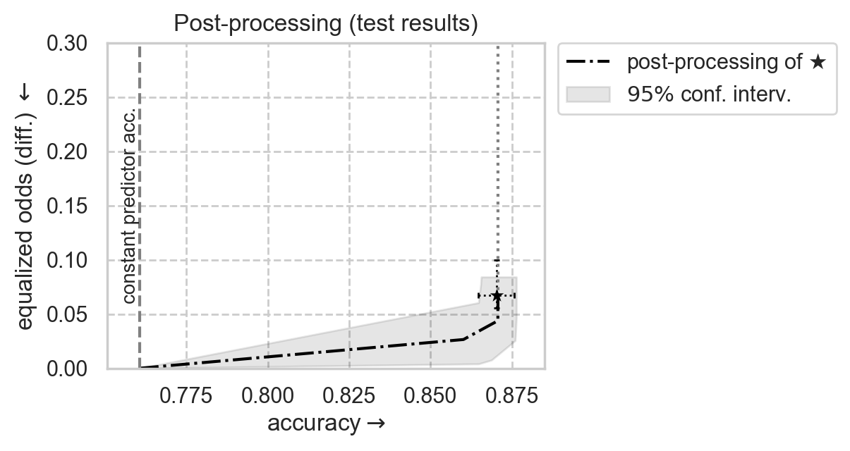
By varying the tolerance (or slack) of the fairness constraint we can map the different trade-offs attainable by the same model (each trade-off corresponds to a different post-processing intervention).
Post-processing fairness methods intervene on the predictions of an already trained model, using different (possibly randomized) thresholds to binarize predictions of different groups.
We’ll be using the `error-parity <https://github.com/socialfoundations/error-parity>`__ package [Cruz and Hardt, 2023].
[11]:
from error_parity.pareto_curve import compute_postprocessing_curve

# Data to fit postprocessing adjustment
fit_data = (X_train, y_train, s_train)
# fit_data = (X_val, y_val, s_val)

# Common kwargs for the `compute_postprocessing_curve` call
compute_postproc_kwargs = dict(
    fit_data=fit_data,
    eval_data={
        "validation": (X_val, y_val, s_val),
        "test": (X_test, y_test, s_test),
    },
    fairness_constraint="equalized_odds",
    tolerance_ticks=np.hstack((
        np.arange(0.0, 0.1, 1e-2),
        np.arange(0.1, 1.0, 1e-1),
    )),
    bootstrap=True,
    n_jobs=N_JOBS,
    seed=SEED,
)

postproc_results_df = compute_postprocessing_curve(
    model=unconstr_clf,
    **compute_postproc_kwargs,
)
Plot post-processing adjustment frontier
[12]:
SHOW_RESULTS_ON = "test"
# SHOW_RESULTS_ON = "validation"

ax_kwargs = dict(
    xlim=(constant_clf_accuracy[SHOW_RESULTS_ON] - 5e-3, 0.885),
    ylim=(0.0, 0.3),
    title="Random Hyperparameter Search (val.)",
    xlabel=PERF_METRIC + r"$\rightarrow$",
    ylabel="equalized odds (diff.) $\leftarrow$" if DISP_METRIC == "equalized_odds_diff" else DISP_METRIC,
)
[13]:
from error_parity.plotting import plot_postprocessing_frontier

# Plot unconstrained model results with 95% CIs
unconstr_performance = unconstr_test_results[f"{PERF_METRIC}_mean"]
unconstr_disparity = unconstr_test_results[f"{DISP_METRIC}_mean"]

sns.scatterplot(
    x=[unconstr_performance],
    y=[unconstr_disparity],
    color="black",
    marker="*",
    s=100,
)

plt.plot(
    (unconstr_test_results[f"{PERF_METRIC}_low-percentile"], unconstr_test_results[f"{PERF_METRIC}_high-percentile"]),
    (unconstr_disparity, unconstr_disparity),
    color="black",
    ls=":",
    marker="|",
    lw=1,
    ms=3,
)

plt.plot(
    (unconstr_performance, unconstr_performance),
    (unconstr_test_results[f"{DISP_METRIC}_low-percentile"], unconstr_test_results[f"{DISP_METRIC}_high-percentile"]),
    color="black",
    ls=":",
    marker="_",
    lw=1,
    ms=3,
)

# Plot postprocessing of unconstrained model
plot_postprocessing_frontier(
    postproc_results_df,
    perf_metric=PERF_METRIC,
    disp_metric=DISP_METRIC,
    show_data_type=SHOW_RESULTS_ON,
    constant_clf_perf=constant_clf_accuracy[SHOW_RESULTS_ON],
    model_name=r"$\bigstar$",
)

# Vertical line with minimum "useful" accuracy on this data
curr_const_clf_acc = constant_clf_accuracy[SHOW_RESULTS_ON]
plt.axvline(
    x=curr_const_clf_acc,
    ls="--",
    color="grey",
)
plt.gca().annotate(
    "constant predictor acc.",
    xy=(curr_const_clf_acc, ax_kwargs["ylim"][1] / 2),
    zorder=10,
    rotation=90,
    horizontalalignment="right",
    verticalalignment="center",
    fontsize="small",

)

# Title and legend
ax_kwargs["title"] = f"Post-processing ({SHOW_RESULTS_ON} results)"
ax_kwargs["xlim"] = (curr_const_clf_acc - 1e-2, 0.885)

plt.legend(
    loc="upper left",
    bbox_to_anchor=(1.03, 1),
    borderaxespad=0)

plt.gca().set(**ax_kwargs)
plt.show()

Let’s train another type of fairness-aware model
In-processing fairness methods introduce fairness criteria during model training.
Main disadvantage: state-of-the-art in-processing methods can be considerably slower to run (e.g., increasing training time by 20-100 times).
We’ll be using the `fairlearn <https://github.com/fairlearn/fairlearn>`__ package [Weerts et al., 2020].
[14]:
from fairlearn.reductions import ExponentiatedGradient, EqualizedOdds

inproc_clf = ExponentiatedGradient(
    estimator=unconstr_clf,
    constraints=EqualizedOdds(),
    max_iter=10,
)
Fit the ExponentiatedGradient [Agarwal et al., 2018] in-processing intervention (note: may take a few minutes to fit).
[15]:
%%time
inproc_clf.fit(X_train, y_train, sensitive_features=s_train)
CPU times: user 49.1 s, sys: 1min 9s, total: 1min 58s
Wall time: 1min 59s
[15]:
ExponentiatedGradient(constraints=<fairlearn.reductions._moments.utility_parity.EqualizedOdds object at 0x16dac2650>,
                      estimator=LGBMClassifier(verbosity=-1), max_iter=10,
                      nu=0.000851617415307666)
In a Jupyter environment, please rerun this cell to show the HTML representation or trust the notebook. On GitHub, the HTML representation is unable to render, please try loading this page with nbviewer.org.
ExponentiatedGradient(constraints=<fairlearn.reductions._moments.utility_parity.EqualizedOdds object at 0x16dac2650>,
                      estimator=LGBMClassifier(verbosity=-1), max_iter=10,
nu=0.000851617415307666)LGBMClassifier(verbosity=-1)
LGBMClassifier(verbosity=-1)
Evaluate in-processing model on test data.
[16]:
from error_parity.evaluation import evaluate_predictions_bootstrap

inproc_test_results = evaluate_predictions_bootstrap(
    y_true=y_test,
    y_pred_scores=inproc_clf.predict(X_test, random_state=SEED).astype(float),
    sensitive_attribute=s_test,
)

print(
    f"In-processing model: \n"
    f">       accuracy = {inproc_test_results['accuracy_mean']:.3}\n"
    f"> equalized odds = {inproc_test_results['equalized_odds_diff_mean']:.3}\n"
)
In-processing model:
>       accuracy = 0.867
> equalized odds = 0.0498
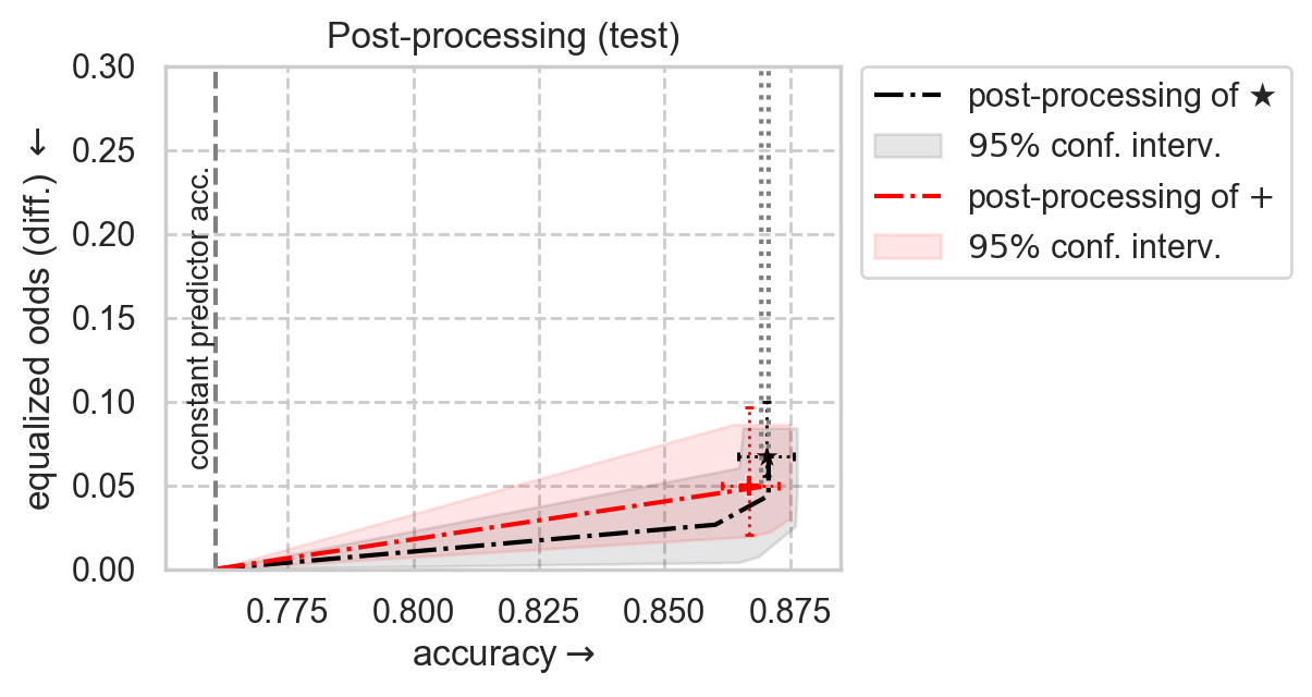
We can go one step further and post-process this in-processing model :)
[17]:
from error_parity.pareto_curve import compute_postprocessing_curve

inproc_postproc_results_df = compute_postprocessing_curve(
    model=inproc_clf,
    predict_method="_pmf_predict",
    **compute_postproc_kwargs,
)
[18]:
# Plot unconstrained model results with 95% CIs
sns.scatterplot(
    x=[unconstr_performance],
    y=[unconstr_disparity],
    color="black",
    marker="*",
    s=100,
)

plt.plot(
    (unconstr_test_results[f"{PERF_METRIC}_low-percentile"], unconstr_test_results[f"{PERF_METRIC}_high-percentile"]),
    (unconstr_disparity, unconstr_disparity),
    color="black",
    ls=":",
    marker="|",
    lw=1,
    ms=3,
)

plt.plot(
    (unconstr_performance, unconstr_performance),
    (unconstr_test_results[f"{DISP_METRIC}_low-percentile"], unconstr_test_results[f"{DISP_METRIC}_high-percentile"]),
    color="black",
    ls=":",
    marker="_",
    lw=1,
    ms=3,
)

# Plot postprocessing of unconstrained model
plot_postprocessing_frontier(
    postproc_results_df,
    perf_metric=PERF_METRIC,
    disp_metric=DISP_METRIC,
    show_data_type=SHOW_RESULTS_ON,
    constant_clf_perf=constant_clf_accuracy[SHOW_RESULTS_ON],
    model_name=r"$\bigstar$",
)

# Plot inprocessing intervention results with 95% CIs
sns.scatterplot(
    x=[inproc_test_results[f"{PERF_METRIC}_mean"]],
    y=[inproc_test_results[f"{DISP_METRIC}_mean"]],
    color="red",
    marker="P",
    s=50,
)

plt.plot(
    (inproc_test_results[f"{PERF_METRIC}_low-percentile"], inproc_test_results[f"{PERF_METRIC}_high-percentile"]),
    (inproc_test_results[f"{DISP_METRIC}_mean"], inproc_test_results[f"{DISP_METRIC}_mean"]),
    color='red',
    ls=":",
    marker="|",
    lw=1,
    ms=3,
)

plt.plot(
    (inproc_test_results[f"{PERF_METRIC}_mean"], inproc_test_results[f"{PERF_METRIC}_mean"]),
    (inproc_test_results[f"{DISP_METRIC}_low-percentile"], inproc_test_results[f"{DISP_METRIC}_high-percentile"]),
    color='red',
    ls=":",
    marker="_",
    lw=1,
    ms=3,
)

# Plot postprocessing of inprocessing model
plot_postprocessing_frontier(
    inproc_postproc_results_df,
    perf_metric=PERF_METRIC,
    disp_metric=DISP_METRIC,
    show_data_type=SHOW_RESULTS_ON,
    constant_clf_perf=constant_clf_accuracy[SHOW_RESULTS_ON],
    model_name=r"$+$",
    color="red",
)

# Vertical line with minimum "useful" accuracy on this data
curr_const_clf_acc = constant_clf_accuracy[SHOW_RESULTS_ON]
plt.axvline(
    x=curr_const_clf_acc,
    ls="--",
    color="grey",
)
plt.gca().annotate(
    "constant predictor acc.",
    xy=(curr_const_clf_acc, ax_kwargs["ylim"][1] / 2),
    zorder=10,
    rotation=90,
    horizontalalignment="right",
    verticalalignment="center",
    fontsize="small",

)

# Title and legend
ax_kwargs["title"] = f"Post-processing ({SHOW_RESULTS_ON})"
ax_kwargs["xlim"] = (curr_const_clf_acc - 1e-2, 0.885)

plt.legend(
    loc="upper left",
    bbox_to_anchor=(1.03, 1),
    borderaxespad=0)

plt.gca().set(**ax_kwargs)

plt.show()
